Hello, welcome to my blog. Apologies for the delay in writing
this post, I have been a little preoccupied lately. Thankfully I am able to
create time to write this post. In this post, I am going to address the problem
of distinguishing images that are ads from non-ads. Concretely, given an image the
goal is to determine if it’s an advertisement (“ad”) or not an advertisement
(“non-ad”). I am going to use the R programming language for this
demonstration.
HANDLING MISSING DATA
In this dataset, the first four attributes contain missing
values i.e. NA. One common way to handle missing data is to completely drop
them from the data and continue the analysis as if these missing observations
were not part of the data in the first place. This is not a very good practice
because it reduces the amount of data one has to work with especially if the
dataset we are using is not very large. In this case, dropping missing data
will reduce the number of observations from N=3279 to N=2359 – this is a loss of
about 28% of the observations. It should be noted that our dataset is not a
particularly large one so dropping missing data may not be such a good idea.
So if we can’t drop missing data how else can we handle them?
Another way is to impute missing values i.e. we try to predict the values of
the missing observations. One method is to impute missing values with the mean
or median of the non-missing observations (for numerical observations) or the
most frequent value (for categorical observations). While these methods help us
to 'predict' missing values it may reduce the predictive accuracy of the model
because we are adding values which may not be correct substitutes for the
missing values.
A superior way of handling missing data is to actually
predict them. That is what I did – I used a random forest model to predict the values
of the missing observations in the dataset. This was done using the missForest
package in R. For other R packages you can use for handling missing data check
out this post.
Next, I randomly split the data into training (75%) and testing
(25%) sets.
BUILDING THE MODEL
I decided to use a Decision tree model and a Logistic
Regression model for this problem. In the following paragraphs I will describe
the procedure I used to build these models.
DECISION TREES
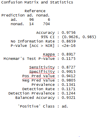
I used the C50 package to build a decision tree model from
the dataset. This was done using the C5.0 function from the C50 package. Next,
I evaluated the model on the test data. The evaluation metrics for the model
are shown below:
 |
| Evaluation metrics for the single decision tree model |
I want to draw your attention to the 4 values I underlined in
red.
- Kappa statistic: Indicates the agreement between the model’s predictions & true values. Ranges from 0 (no agreement) to 1 (perfect agreement).
- Sensitivity: This measures the proportion of positive examples that were correctly classified. Also known as the true positive rate or recall.
- Pos Pred Value: This is the fraction of predicted positive examples that were actually positive. Also known as precision.
- Specificity: This measures the proportion of negative examples that were correctly classified. Also known as true negative rate.
We can see that the above values for this decision tree model
are pretty good indicating that it does quite a good job of discriminating
between images that are ads vs non ads.
Although these values looked good, I felt they could be
better so I built a boosted decision tree model from the data. This was done by
passing ‘trials’ = 10 to the C5.0 function – this generated 10 weak learners
from the dataset. The evaluation metrics for the model are shown below:
 |
| Evaluation metrics for the Boosted Decision tree model |
Next, I tried different values of ‘trials’ via parameter
tuning with the caret package form R. 8 candidate models were tested and the
best model was selected based on the Kappa statistic. The best model was the
model with trials = 20 i.e. 20 weak learners. The evaluation metrics for this
model is given below:
 |
| Evaluation metrics for the best model |
LOGISTIC REGRESSION
Before I talk about how I built the logistic regression
model, let me give some preliminary details. I noticed that the dataset had a
relatively large number of features compared to the number of observations
which could lead to overfitting i.e. good
performance on the training data but poor performance on the test data. In
order to combat this problem, I performed regularization
with the following goals in mind:
- Feature selection – I used regularization to select the best subset of features that were able to give good predictive accuracy.
- I also used regularization to ensure that the feature coefficients did not get too large as this is a sign of overfitting.
I used the glmnet package to build regularised logistic
regression model from the data. Next, I evaluated the model on test data. I
evaluated 3 sets of predictions for 3 values of lambda used by the model – 10-5,
10-4 and 10-3. Lambda is a value used to control the size of the coefficients for the logistic regression model. The evaluation metrics for these
predictions are shown below:
 |
| Evaluation metrics for lambda = 0.0001 |
 |
| Evaluation metrics for lambda = 0.001 |
 |
| Evaluation metrics for lambda = 0.01 |
From this we can conclude that the best regularized logistic
regression model is the one with lambda = 0.001.
CONCLUSION
Before I write my conclusion, I want to highlight the
importance of properly handling missing observations. If we had merely dropped
the missing observations it is unlikely that we would achieve the impressive
evaluation metrics we obtained in this demonstration.
So which model is better? The best decision tree model had a
Kappa statistic of 0.9033 while the best regularized logistic regression model
had a Kappa statistic of 0.9014. They also have similar values for the other
evaluation metrics so I think I will call it a tie. Do you have a different
opinion? Let me know!!
SUMMARY
In this post, I demonstrated how we can discriminate between
images that are ads or non-ads using a decision tree model and a logistic
regression model. You can find the code for this post on my GitHub repository. Thank you for reading this post, as always if you have any questions or
comments feel free to leave a comment and I will answer you. Once again subscribe to my blog in case you have not. Have a great week
ahead and Ramadan Kareem to all my Muslim readers. Cheers!!!
No comments:
Post a Comment